3 Strain
Introduction
Click to expand
In Chapter 2 we learned how to calculate normal and shear stresses with respect to a plane of interest, such as a cross-sectional area or an inclined plane. If stresses get too large the object will break, so it is important that engineers design structures and machines such that the stresses stay within certain acceptable limits. It is also important that objects do not deform so much that they are no longer fit for their original purpose. Strain is a measure of the intensity of a deformation—that is, the deformation per unit length.
Imagine two points on a body, A and B separated by some distance L (Figure 3.1). In statics (and dynamics), objects are assumed to be rigid and they do not deform when subjected to forces. In reality, forces will cause an object to deform and its dimensions will change. As points A and B move with the object, the distance between them will change to some new distance L’.
These deformations may be very large relative to the size of the object (e.g., a rubber band) or they may be relatively small (e.g., structural members) but there will always be some amount of deformation as no material is infinitely stiff, as we will learn in Chapter 4. Engineers must design structures and machines such that these deformations are not excessively large for the intended application.
This chapter will introduce two types of strain. Section 3.1 covers normal strain which, like normal stress, occurs when objects are subjected to axial loads. Section 3.2 covers shear strain which, like shear stress, occurs when objects are subjected to shear loads.
3.1 Normal Strain
Click to expand
A simple example of normal strain is the deformation of a bar subjected to an axial load. Consider a bar of length L subjected to a tensile axial load P as shown in Figure 3.2. The load will create a normal stress in the rod and will also cause the rod to elongate by an amount ΔL.
If the same load were applied to a longer rod of length 2L with the same cross-sectional area, the longer rod will elongate by an amount 2ΔL. The deformation depends on the original length of the rod in this case, but the strain does not. Strain is a measure that normalizes the change in length by the original length. Normal strain is defined as:
\[ \boxed{\varepsilon=\frac{\Delta L}{L}} \tag{3.1}\]
ε = Normal strain
ΔL = Change in length [mm, in]
L = Original length [mm, in]
This is a normal strain because it occurs under axial load and is associated with a change in length of the object. Since normal strain is defined by dividing one length by another it does not have any units. However, it is fairly common to still include units of mm/mm or in/in.
For example, if the rod was initially 5 m long and it elongated by 12 mm, the normal strain can be calculated as:
\[ \varepsilon=\frac{\Delta L}{L}=\frac{12}{5,000}=0.0024{~mm} /{mm}=0.0024 \]
Note that the units used for ΔL and L must be the same, but it does not matter if they are expressed in mm or m. Using meters instead yields the same answer:
\[ \varepsilon=\frac{\Delta L}{L}=\frac{0.012}{5}=0.0024{~m}/{m}=0.0024 \]
Because strains tend to be quite small in many engineering applications, they are sometimes expressed with a prefix to eliminate the leading zeros. For example, a strain of 0.0024 may be expressed as 2.4 mm/m or 2400 µm/m or simply 2400 µ. Strains may also be expressed as a percentage, which can be found simply by multiplying the strain by 100%. The below strains are all equivalent:
\[ \varepsilon=0.0024{~mm}/{mm}=0.0024{~m}/{m}=0.0024=2.4{~mm}/{m}=2400~\mu{m}/{m}=2400 ~\mu=0.24\% \]
We will continue to use the sign convention that we defined for normal stress. Tensile forces and stresses, which are associated with elongation of the bar and tensile normal strain, are positive. Compressive forces and stresses, which are associated with shortening of the bar and compressive normal strain, are negative (Figure 3.3).
See Example 3.1 for a problem involving a bar experiencing both tension and compression. Example 3.2 involves strain in two parallel cables.
Example 3.1
The bar is subjected to forces F1 = 30 kips and F2 = 10 kips as shown. Segment AB is originally 10 inches in length and segment BC is originally 15 inches in length. As a result of the applied forces, the normal strain in segment AB is – 0.03 in/in and the strain in segment BC is 0.045 in/in.
- Determine the change in length of each segment
- Determine the overall strain for the entire bar
Example 3.2
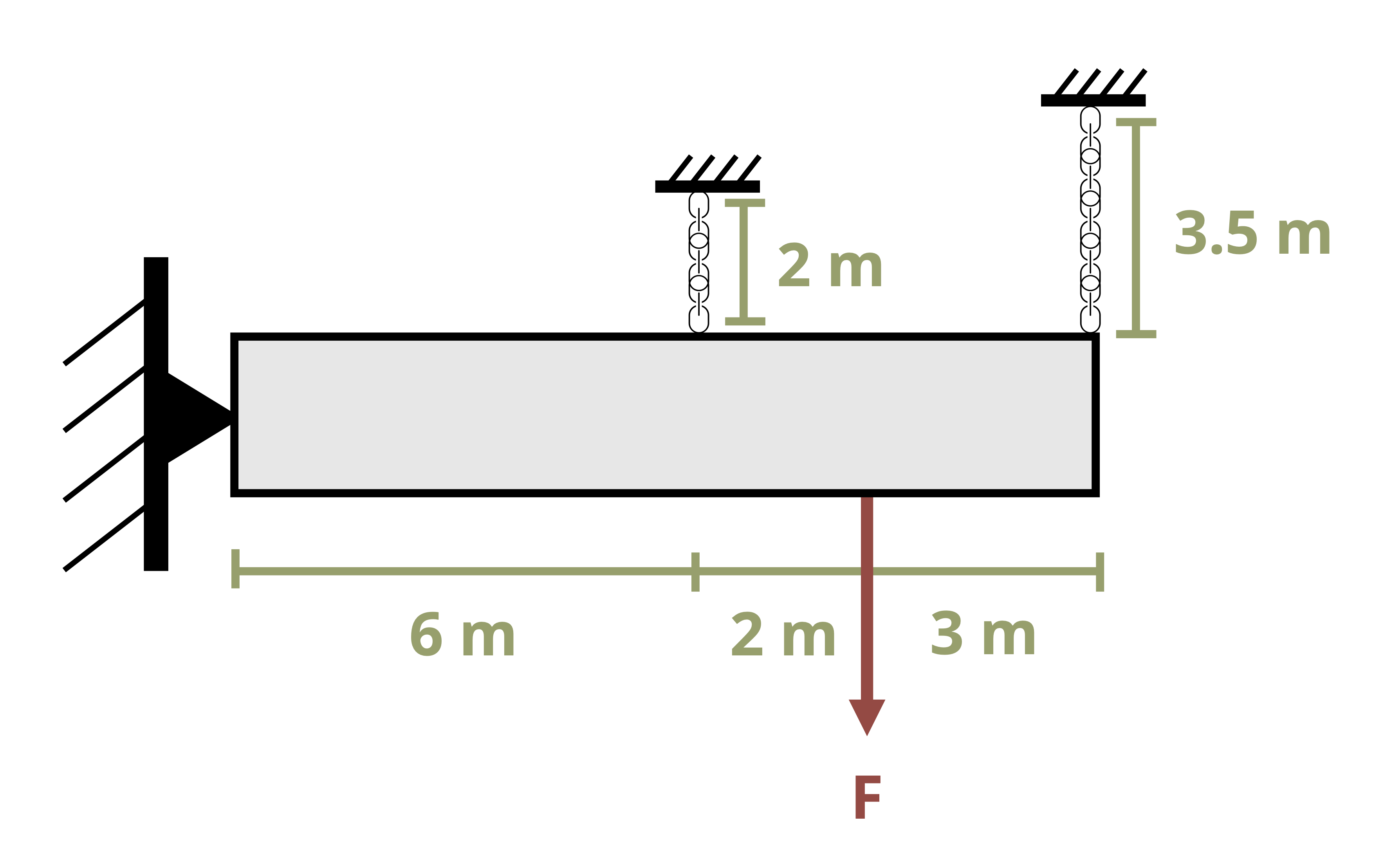
Rigid bar ABCD is supported by a pin at A and cables at B and D. After load F is applied, the strain in cable D is 2300 µm/m. Determine the strain in cable B.
Consider the deflected position of rigid bar ABCD. We can calculate the change in length of cable D.
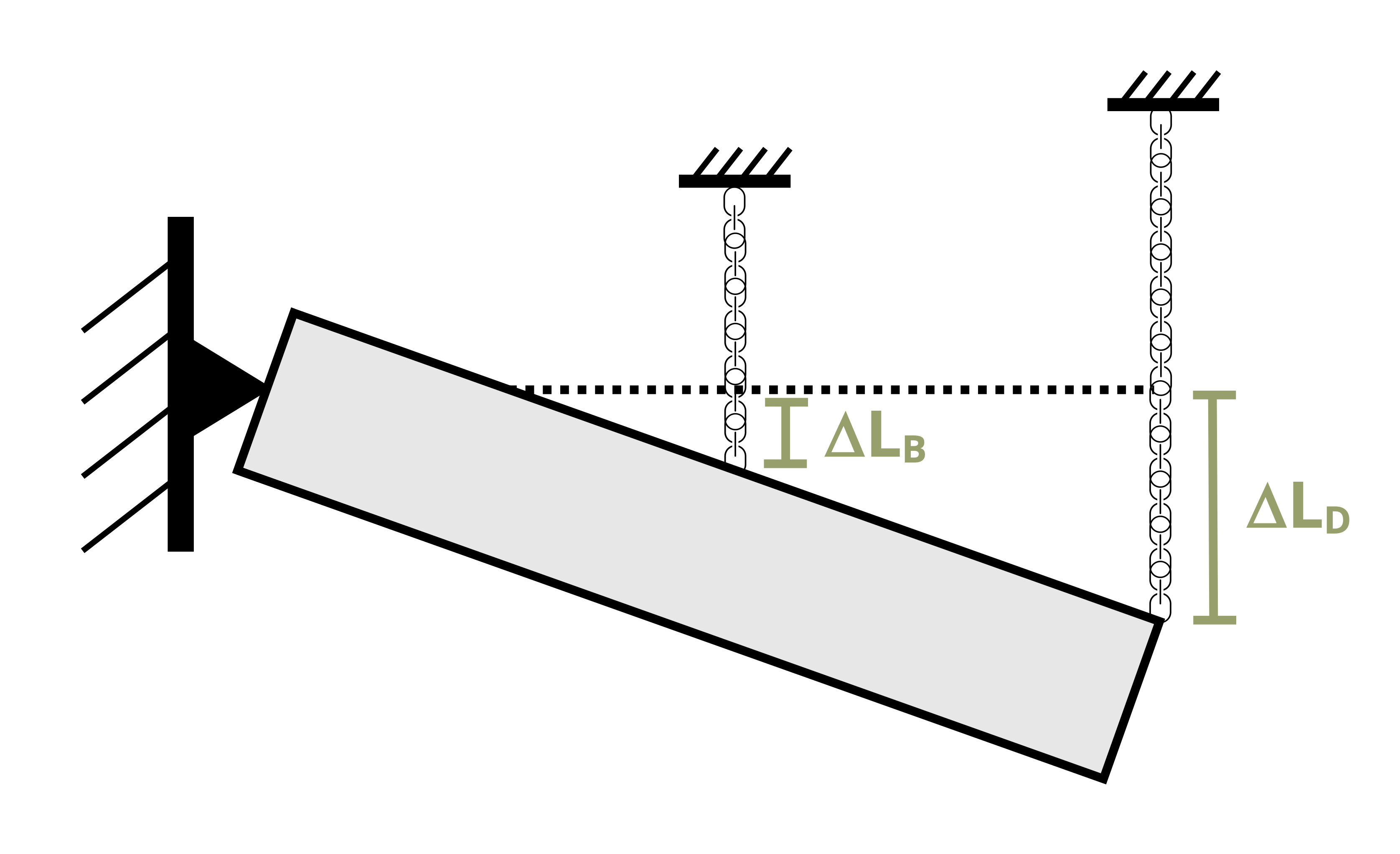
\[ \Delta L_D=\varepsilon L=2300 \times 10^{-6} * 3.5{~m}=0.00805 {~m}=8.05 {~mm} \]
Point D will deflect downwards by 8.05 mm. Use similar triangles to find the deflection of point B.
\[ \begin{gathered} \frac{\Delta L_B}{6{~m}}=\frac{8.05{~mm}}{11{~m}} \\ \Delta L_B=\frac{6{~m} * 8.05{~mm}}{11{~m}}=4.39{~mm} \end{gathered} \]
Cable B will elongate by 4.39 mm. Use this to determine the strain in cable B. Be careful to be consistent with units. Either use ΔL = 4.39 mm and L = 2000 mm, or ΔL = 0.00439 m and L = 2 m.
\[ \varepsilon=\frac{\Delta L}{L}=\frac{4.39{~mm}}{2000{~mm}}=0.002195{~m}/{m}=2195 ~\mu{m} /{m} \]
3.2 Shear Strain
Click to expand
Consider a small, square element that may be part of a body such as that shown in Figure 3.1. As well as the distance between points changing as the body deforms, the shape of this square element will also change. The corners of the square element will initially form right-angles. As the body deforms and the points move with the object, the shape of the element changes and the corners no longer form right-angles (Figure 3.4).
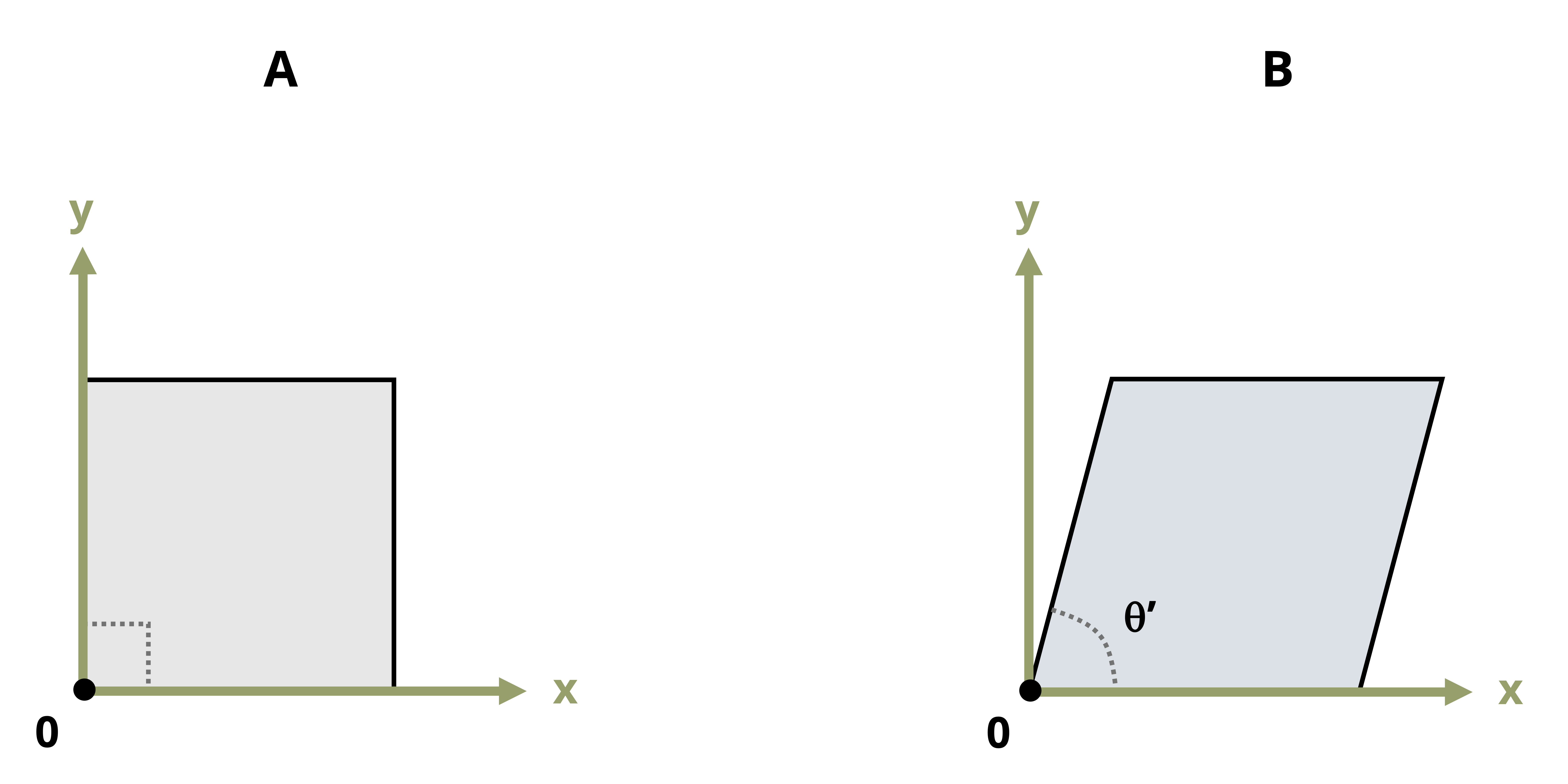
While normal strain represents a change in length, a shear strain represents a change in angle—a distortion of the shape. Specifically, provided we start with right-angled corners, shear strain is defined as the original angle (before deformation) minus the new angle (after deformation). Regardless of the shape of the body, a square element can always be defined such that the original angle is always a right angle. After deformation, the new angle between these three points is 𝜃’. Shear strain is given the symbol γ and is, like normal strain, a dimensionless quantity, so is represented in radians (not degrees). Thus the original right angle is represented as \(\frac{\pi}{2}\) radians and the shear strain as:
\[ \boxed{\gamma=\frac{\pi}{2}-\theta^{\prime}} \tag{3.2}\]
𝛾 = Shear strain [rad]
\(\frac{\pi}{2}\) = Original angle [rad]
𝜃’ = New angle [rad]
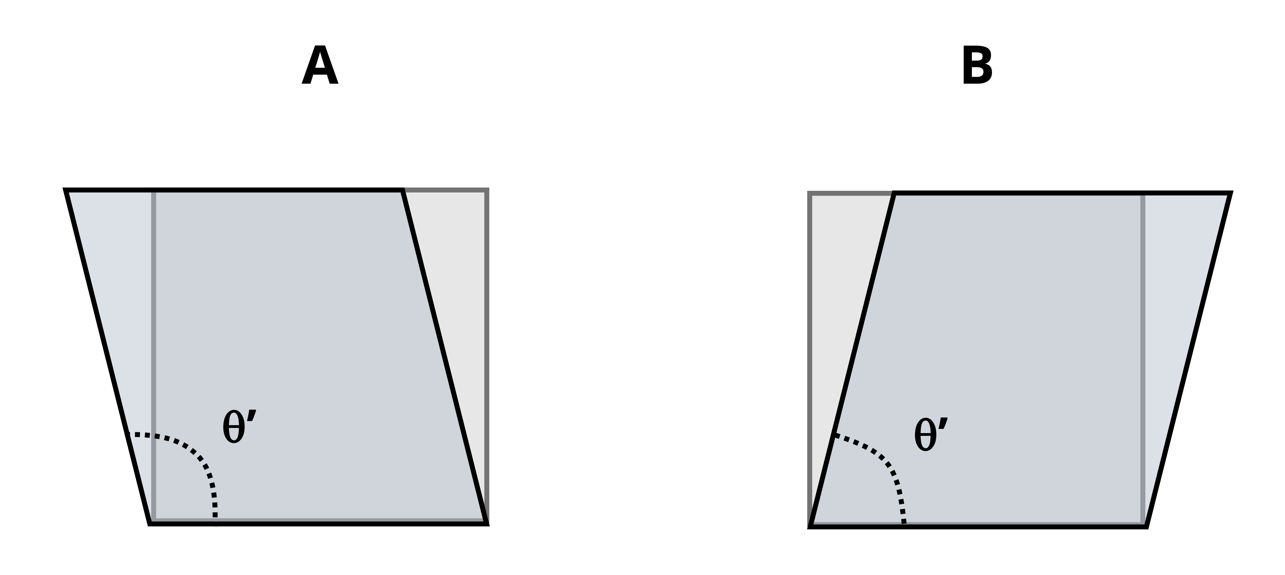
Since we always subtract the new angle from the original angle, note that if the angle increases we get a negative shear strain and if the angle decreases we get a positive shear strain (Figure 3.5).
See Example 3.3 and Example 3.4 to practice calculating shear strain.
Example 3.3
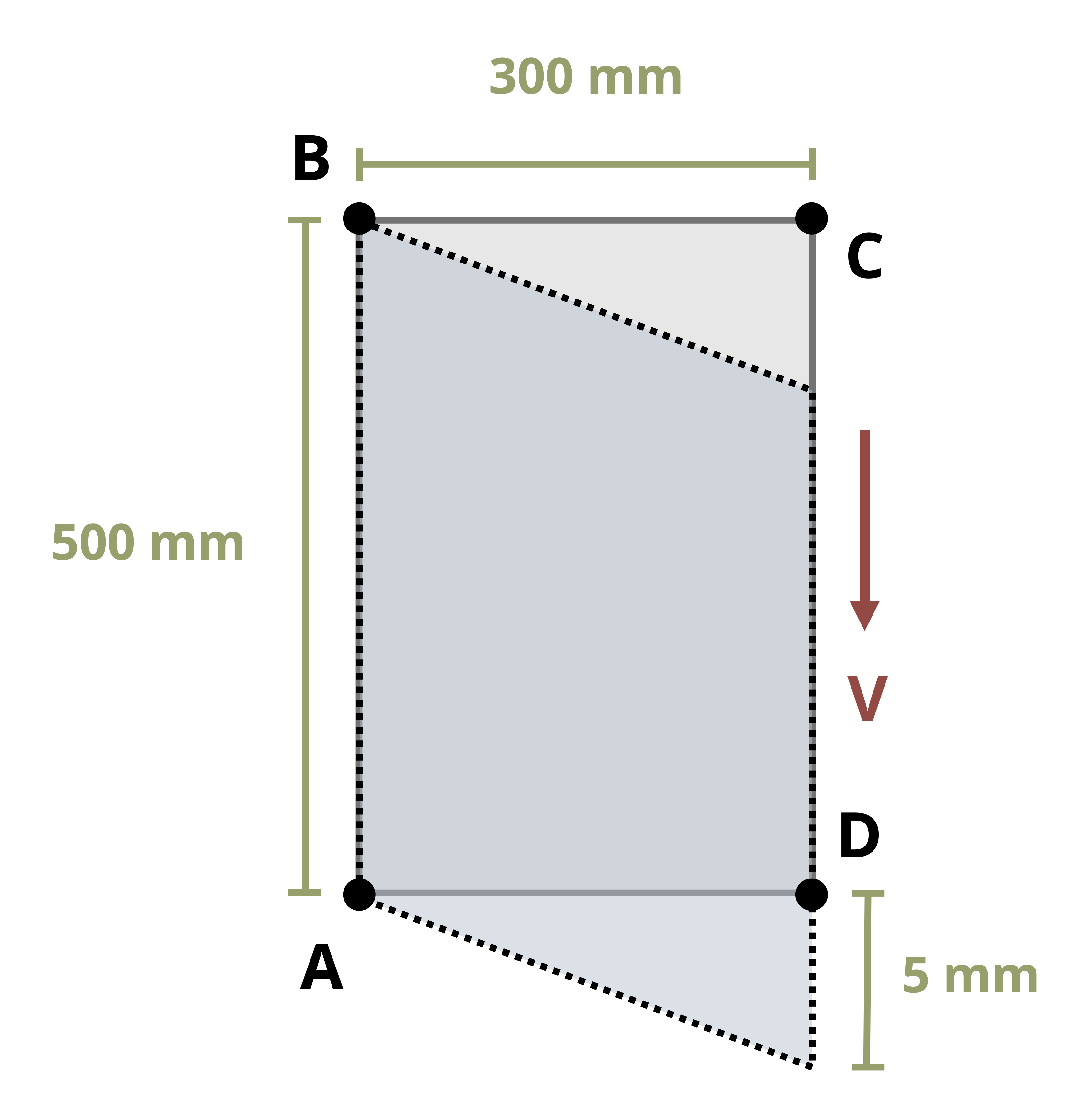
A thin rectangular plate has a base of 300 mm and a height of 500 mm. Initially corners A, B, C, and D are all right-angles. The plate is subjected to a shear force V which deforms the plate into the dotted lines shown. Corner D moves straight downward by 5 mm. Determine the shear strain at corner A.
We could calculate the new angle at corner A as \(\theta^{\prime}=\frac{\pi}{2}+\alpha\).
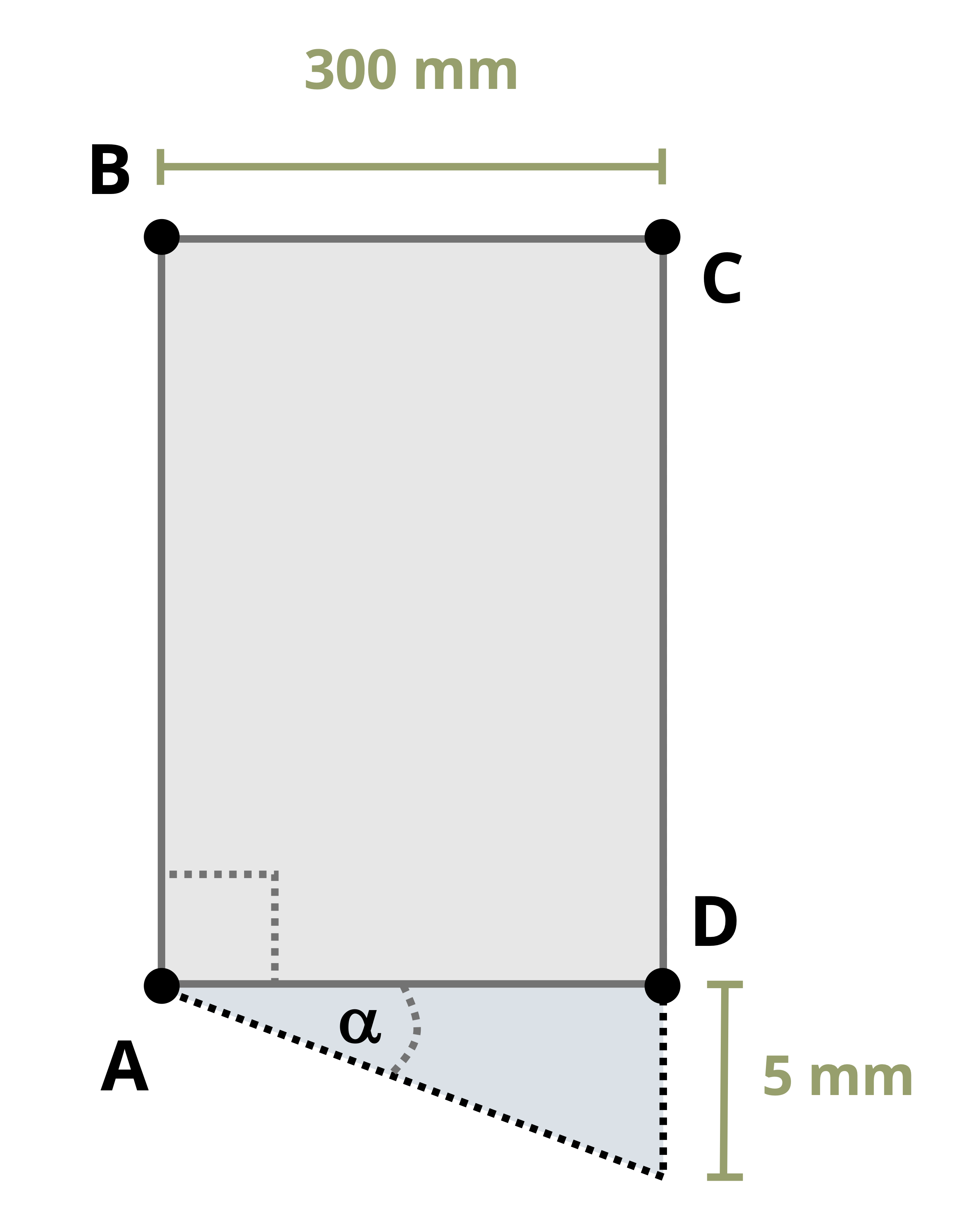
Angle α can be found since there is a triangle of base 300 mm and height 5 mm.
\[ \alpha=\tan ^{-1}\left(\frac{5}{300}\right)=0.01667 {~rad} \]
Then:
\[ \theta^{\prime}=\frac{\pi}{2}+0.01667{~rad}=1.5875 {~rad} \]
Now the shear strain can be calculated:
\[ \gamma=\frac{\pi}{2}-\theta^{\prime}=\frac{\pi}{2}-1.5875{~rad}=-0.01667 {~rad} \]
Notice that this is just the negative of angle α. Since the shear strain is the change in angle and α represents the increase of the angle, we could have simply said that angle α is the shear strain. As defined in Section 3.2, the shear strain is negative because the angle is increasing.
Example 3.4
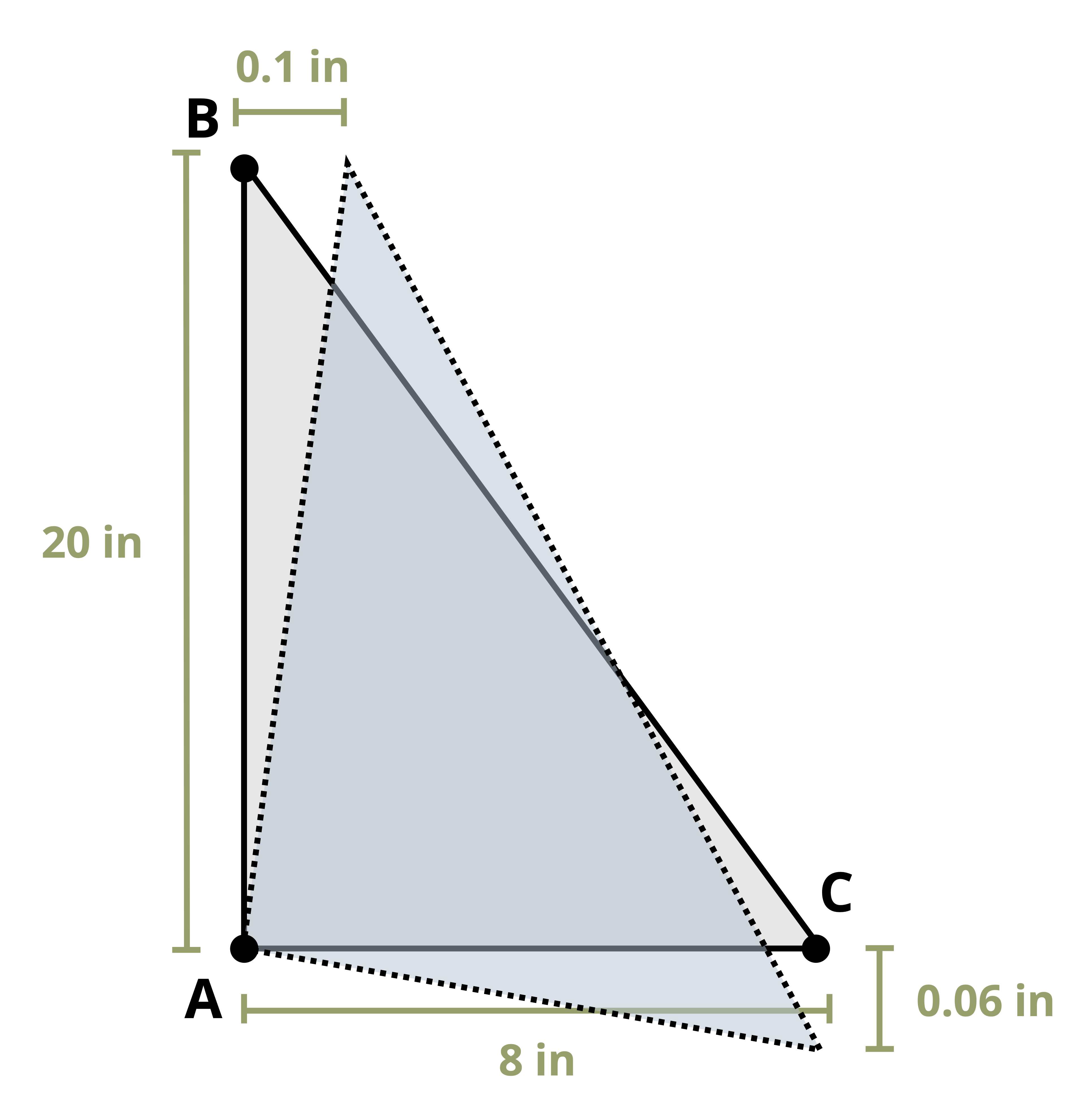
A thin triangular plate ABC has a base of 8 inches and a height of 20 inches. Corner A is initially a right-angle. When subjected to a shea load, the plate deforms as shown. Corner B moves 0.1 inches to the right and corner C moves 0.06 inches downward. Determine the shear strain at corner A.
The angle at A will decrease by angle α and increase by angle β. Start by finding these angles.
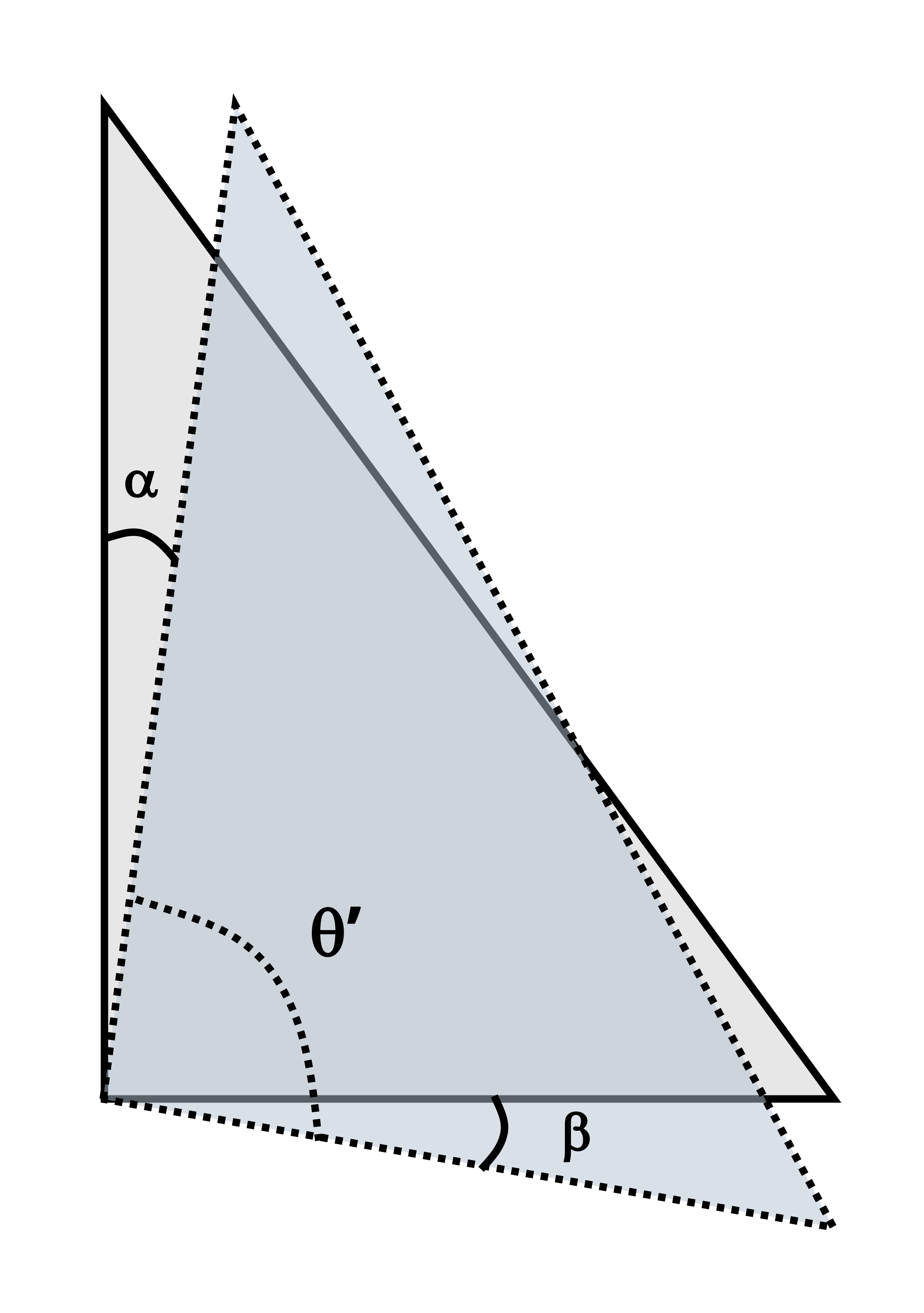
\[ \begin{gathered} \alpha=\tan ^{-1}\left(\frac{0.1}{20}\right)=0.005{~rad} \\ \beta=\tan ^{-1}\left(\frac{0.06}{8}\right)=0.0075{~rad} \end{gathered} \]
The new angle at A will be:
\[ \theta^{\prime}=\frac{\pi}{2}-\alpha+\beta=1.5708-0.005+0.0075=1.5733{~rad} \]
With the new angle known, we can calculate the shear strain.
\[ \gamma=\frac{\pi}{2}-1.5733{~rad}=-0.0025{~rad} \]
Note that we could have calculated the shear strain more directly. Since shear strain is just the change in angle, we could have said that the angle at A decreases by angle α and increases by angle β.
Recall that shear strain is positive if the angle decreases and negative if the angle increases. The change in angle at A, and thus the shear strain, could be calculated as:
\[ \gamma=\alpha-\beta=0.005{~rad}-0.0075{~rad}=-0.0025{~rad} \]